Davide Dametti
Benchmarking in Time Series Forecasting
Introduction
Before training any model in time series forecasting, it is essential to establish benchmarks that serve as a reference for performance comparison.
These benchmarks are simple models that are intuitive, easy to implement, and quick to train. The primary objective is that any more complex model should at least outperform these benchmarks to justify its use.
Benchmarking is a crucial initial step, as even the simplest models can be difficult to surpass. For instance, in the 5th edition of the Makridakis Competitions, only 48% of participating teams managed to outperform the naive prediction (which we define below), and only 7.5% of teams surpassed all benchmarks set by the competition organizers.
Therefore, before investing time, money, and computational resources into complex models, it is important to ensure they deliver superior performance compared to these benchmarks.
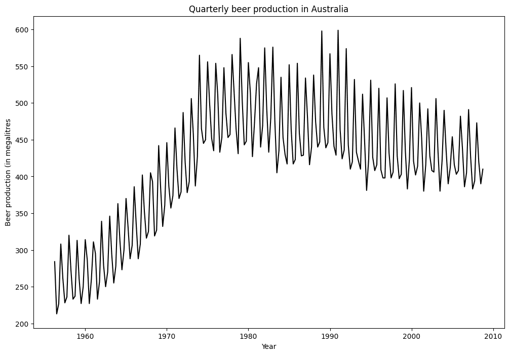
Below is a non-exhaustive list of simple benchmarks for time series forecasting; to illustrate them, we will use the ausbeer dataset, available in the pmdarima package.
import numpy as np
import pandas as pd
import matplotlib.pyplot as plt
from pmdarima.datasets import load_ausbeer
# Load the ausbeer dataset
data = load_ausbeer()

# Create a time index and convert to dataframe
date_range = pd.date_range(start='1956-03-01', end='2009-03-01', freq='Q')

df = pd.DataFrame(data, columns=["value"], index=date_range)

# Train-test split
cutoff_date = pd.Timestamp("2007-09-30")

train = df[df.index < cutoff_date]
test = df[df.index >= cutoff_date]
Benchmarks
Historical Mean
As the name suggests, this method predicts future values as the mean of the historical time series.
For time series with trends, it may be beneficial to use only recent data to compute the mean, as assigning equal weight to older and newer values might not be ideal.
historic_mean_pred = [train['value'].mean()] * len(test)
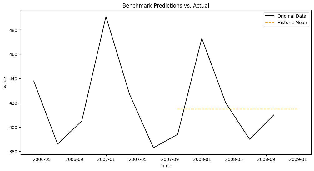
The chart shows a detail of the last years only, from 2006 onward.
Naive prediction
The naive benchmark predicts future values by simply assuming they will be equal to the last observed value.
This approach may not be suitable for series with strong trends or seasonal cycles, as it does not capture such patterns.
naive_pred = [train['value'].iloc[-1]] * len(test)
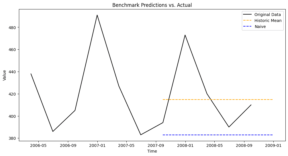
The chart shows a detail of the last years only, from 2006 onward.
Drift Method
The drift method extends the naive approach by incorporating a trend component. It assumes that future values will continue to change at the same average rate as observed in the past.
This method is particularly useful for time series with consistent upward or downward trends. However, if the trend changes direction over time, the drift method may become inaccurate, as it assumes that past trends will continue indefinitely.
Also, this method works by identifying the overall trend between the earliest and latest data points, then extending that trend forward to make future predictions. This means that, if the time series follows a seasonal pattern, it is important to ensure that the first and last observations belong to the same period in the cycle; otherwise, the inferred trend may be misleading.
from sktime.forecasting.naive import NaiveForecaster

forecaster = NaiveForecaster(strategy="drift")
forecaster.fit(train['1980-06-30':])

drift_pred = forecaster.predict(fh=list(range(1, len(test) + 1)))
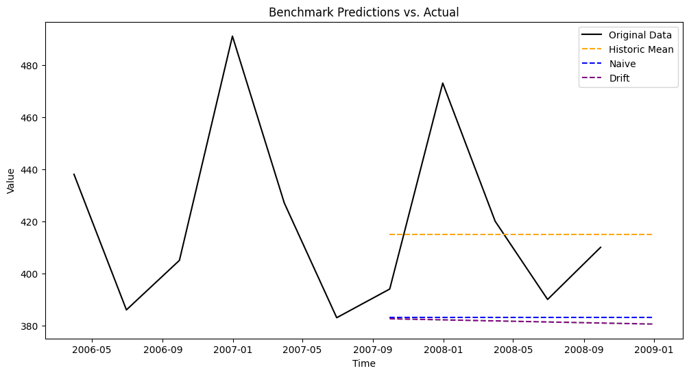
The chart shows a detail of the last years only, from 2006 onward.
Seasonal Naive prediction
The seasonal naive benchmark is used for time series that exhibit repeating patterns over fixed time intervals, such as daily, weekly, or yearly cycles. It makes predictions by assuming that future values will be the same as those observed in the corresponding period of the previous cycle.
seasonality = 4
seasonal_naive_pred = train['value'].iloc[-seasonality:].tolist()
seasonal_naive_pred = (seasonal_naive_pred * (len(test) // seasonality + 1))[:len(test)]
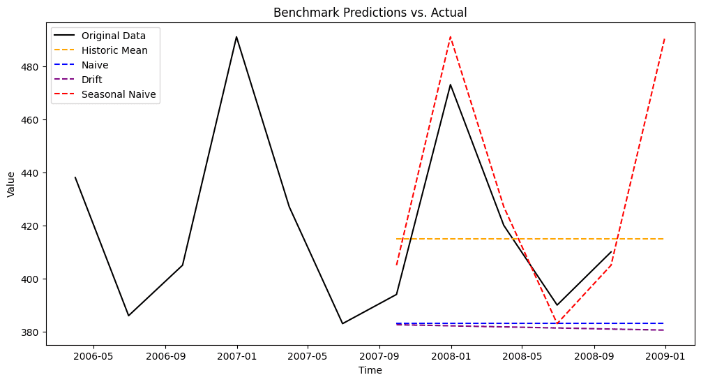
The chart shows a detail of the last years only, from 2006 onward.
Other Benchmarks
While we have defined benchmarks as simple and easy-to-train models, other approaches can serve a similar purpose: providing quick predictions that are easy to implement and setting a baseline for model evaluation.
Both Python and R offer automated tools that identify optimal parameters for popular modeling techniques through search algorithms. These can also function as benchmarks, as they are relatively fast to train and yield reliable forecasts.
AutoETS
The AutoETS class from the Python package sktime automatically selects the best model from the ETS family through parameter tuning.
from sktime.forecasting.ets import AutoETS
auto_ets = AutoETS(auto=True, sp=4)  # sp=4 for seasonality of 4
auto_ets.fit(train['value'])
ets_pred = auto_ets.predict(test.index)
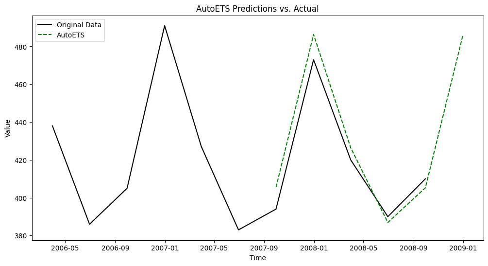
The chart shows a detail of the last years only, from 2006 onward.
AutoARIMA
Similarly, the auto_arima function from the Python package pmdarima finds the optimal parameters for an ARIMA model automatically.
arima_model = auto_arima(train['value'], seasonal=True, m=4, stepwise=True)

n_test = len(test)
arima_pred = arima_model.predict(n_periods=n_test)
arima_pred_series = pd.Series(arima_pred, index=test.index)
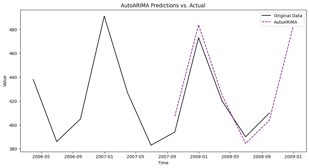
The chart shows a detail of the last years only, from 2006 onward.
References
- The results of the M5 competition can be found here. More on the Makridakis competitions can be found on the corresponding Wikipedia page.
- The documentation for the sktime's AutoETS class is here.
- The documentation for the pmdarima's auto_arima function is here.